

End Effect and Electromagnetic Force Characteristics of Two Adjacent Linear Induction Motors
-
摘要:
直线感应电机在中低速磁浮列车应用中两两相邻,磁场相互干涉. 为探究磁场干涉对相邻电机电磁力特性的影响,首先,基于麦克斯韦方程组建立相邻电机各区域矢量磁位方程,利用边界条件对各区域矢量磁位进行求解;然后,推导得到相邻电机气隙磁场、牵引力和法向力表达式,分析相邻电机磁场干涉对电机电磁力的影响,并利用有限元仿真对理论模型进行检验;最后,研究电机间距和滑差频率对相邻电机电磁力的影响. 研究结果表明:2台电机边端效应引起的行波相互影响,前一台电机(LIM1)受后一台电机(LIM2)影响较小,而LIM2则受LIM1影响较大;LIM2牵引力和法向力均随间距的变化产生波动,间距越小,滑差频率也越小,波动幅度越大,LIM2电磁力受间距影响波动幅度越大;当滑差频率为8 Hz、速度为160 km/h、电流为400 A时,LIM2牵引力相较LIM1最大可增加83%;LIM2法向力最大可减小6.6 kN,将大大减轻悬浮系统的负担.
Abstract:Objective The medium and low speed maglev is driven by linear induction motors (LIMs), which are composed of finite-length primary winding and infinite-length secondary induction rail. This configuration offers several advantages, including structural simplicity, low construction costs, and ease of maintenance. However, the structural characteristics of a discontinuous primary and a continuous secondary plate result in mutual interference of secondary eddy currents at adjacent positions. This interference alters the air-gap magnetic field of the motor, which directly impacts both the traction force and the normal force of the motor. To elucidate the influence characteristics and underlying mechanisms of adjacent motor configurations on electromagnetic forces, enhance motor traction performance, and address issues related to the normal force, this study focused on two adjacent and series-connected LIMs. Theoretical and simulation models were developed to investigate the effects of two key factors, including the motor spacing and slip frequency, on the traction and normal forces of the two motors.
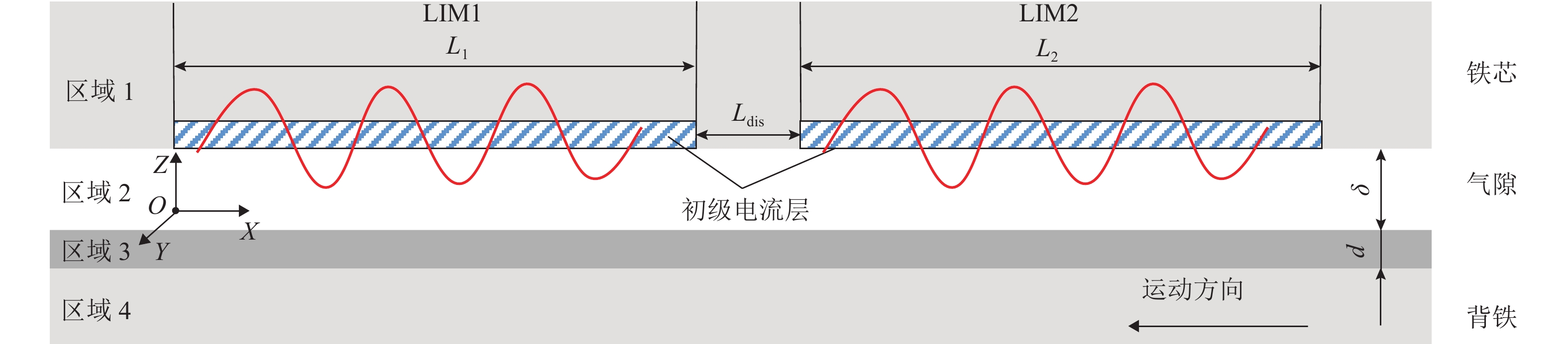
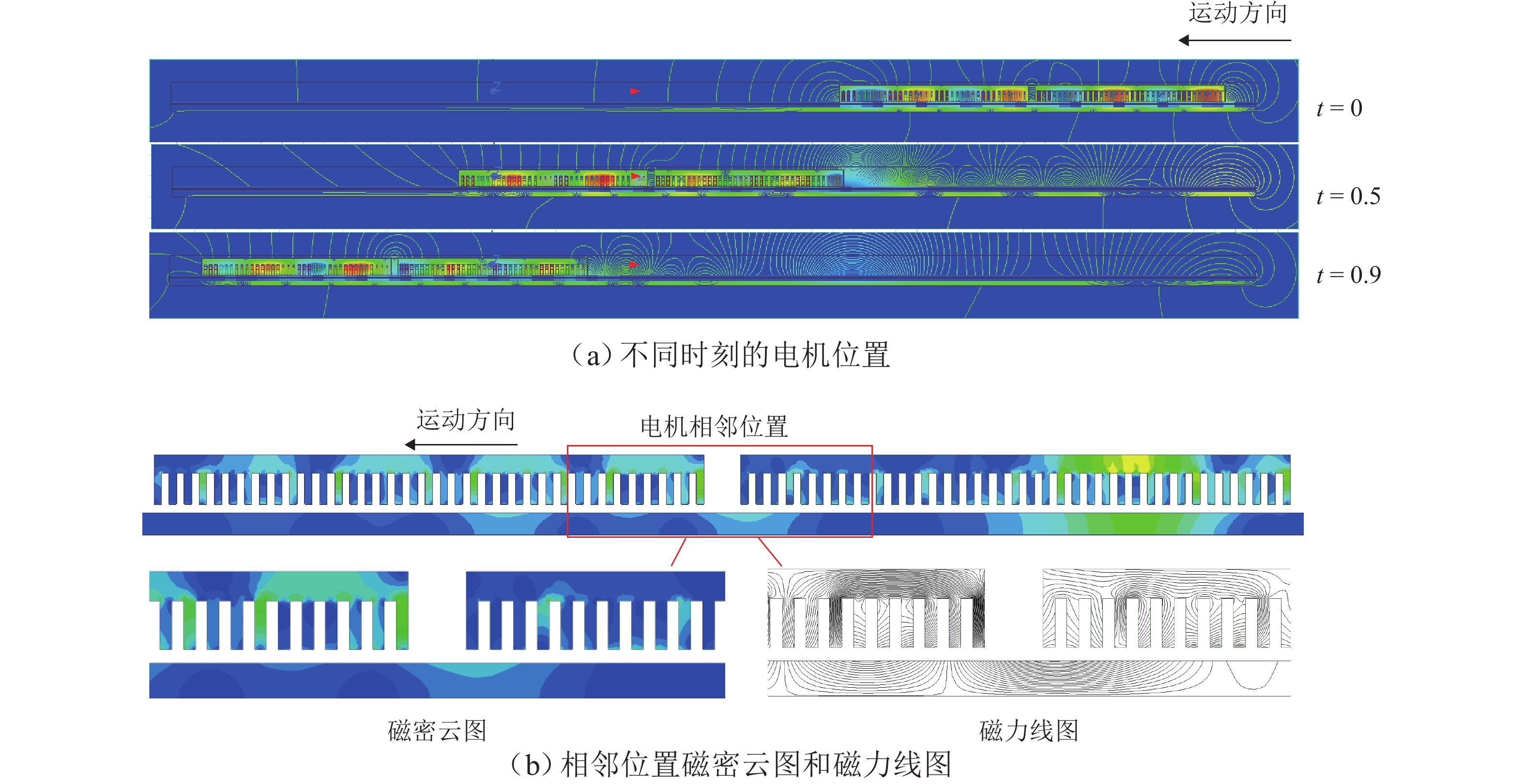
Methods To investigate the influence of adjacent LIM arrangements on electromagnetic forces in medium and low speed maglev and gain a deeper understanding of the magnetic field interference between two LIMs, as well as its intrinsic effects on electromagnetic forces, firstly, vector magnetic potential equations were established for each region of the adjacent motors based on Maxwell’s equations, and the two-dimensional vector magnetic potential for each region was solved by using boundary conditions. Secondly, the expressions for the air-gap magnetic field, traction force, and normal force of the two LIMs were derived based on the air-gap vector magnetic potential and the distribution of primary currents. These expressions were used to analyze the characteristics and underlying mechanisms of how magnetic field interference between adjacent motors affects electromagnetic forces. Thirdly, a finite element analysis (FEA) model of two adjacent motors was developed by using Maxwell software to calculate the electromagnetic forces under different motor spacings. The simulation results were compared with theoretical predictions to validate the accuracy of the theoretical calculation method. Finally, the established theoretical model was utilized to explore the effects of two critical factors, including motor spacing and slip frequency, on the electromagnetic forces of the adjacent motors. By analyzing the air-gap magnetic field under various operating conditions, the study revealed the intrinsic mechanism by which the electromagnetic force of LIM2 was influenced by motor spacing.
Results The variation trends of the traction force between the two motors, as calculated through both theoretical and finite element simulation methods, exhibit a high degree of consistency, thereby validating the accuracy of the theoretical model. In the boundary conditions of the theoretical model, the magnetic permeability of the iron core and back iron is assumed to be infinite, and the primary current is approximated as a thin layer. Consequently, the theoretical calculations yield slightly larger fluctuations in the traction force of LIM2 with respect to motor spacing compared to the simulation results. From the expression of the air-gap magnetic field of the motor, the backward traveling wave caused by the end effect at the exit of LIM1 is influenced by factors such as the primary current, slip frequency, and motor spacing of LIM2. Similarly, the forward traveling wave caused by the end effect at the entry of LIM2 is affected by the parameters of LIM1 and the spacing between the two motors. Consequently, the air-gap magnetic field of the linear motor is altered due to the influence of the adjacent motor. The impact of adjacent motor arrangements on the longitudinal air-gap magnetic field is relatively minor, whereas the effect on the vertical air-gap magnetic field is more pronounced. This influence leads to corresponding variations in the motor’s traction force and normal force. As the motor is less affected by the backward traveling wave induced by the exit-end effect and more significantly affected by the forward traveling wave induced by the entry-end effect, LIM1 is less affected by LIM2, whereas LIM2 is more significantly influenced by LIM1. The computational results indicate that the traction force of LIM1 is nearly unaffected by motor spacing and exhibits minimal variation under different slip frequencies. For various slip frequencies, the operating speed and input current of LIM1 remain consistent, resulting in negligible differences. In contrast, for LIM2, as the slip frequency is smaller, its traction force is more significantly influenced by motor spacing. As the spacing increases, the amplitude of traction force fluctuations for LIM2 decreases across all slip frequencies. When the slip frequency is 8 Hz, and the spacing is 1.5 times the pole pitch, the traction force of LIM2 reaches 8.4 kN, which is 1.83 times that of LIM1 (4.6 kN), representing an 83% increase. Conversely, when the spacing is reduced to 0.6 times the pole pitch, the traction force of LIM2 drops to 0.6 kN, which is merely 13% of LIM1’s traction force, signifying an 87% reduction. These results underscore the importance of spacing design in optimizing the traction performance of LIM2. Furthermore, as the slip frequency decreases, the normal force of LIM1 increases. However, the normal force of LIM1 is almost unaffected by the motor spacing at different slip frequencies. In contrast, the normal force of LIM2 exhibits fluctuations with varying spacing under different slip frequencies. Smaller spacing and slip frequencies lead to a greater impact on the normal force of LIM2. A well-designed motor spacing can effectively reduce the normal force of LIM2, thereby enhancing the stability of maglev vehicles. When the slip frequency is 8 Hz, and the motor spacing is 2.1 times the pole pitch, the normal force of LIM2 is 1 kN, which is 6.6 kN lower than that of LIM1 measured at 7.6 kN. This reduction translates to a weight decrease of 660 kg per motor for the levitation system. However, when the motor spacing is reduced to 1.2 times the pole pitch, the normal force of LIM2 rises dramatically to 28.2 kN, which is 3.7 times greater than that of LIM1, representing a 270% increase. This additional force imposes approximately two tons of extra load on the levitation system per motor.
Conclusion The electromagnetic force of a rear-positioned LIM is significantly influenced by the presence of a front-positioned LIM, as well as the spacing between the motors. However, the optimal spacing for achieving the desired traction force and normal force varies under different operating conditions and system requirements. Therefore, in practical engineering applications, both the traction demands and levitation capabilities of the vehicle should be considered for the design of the motor spacing. The findings can provide theoretical guidance and technical support for the application of LIMs in medium and low speed maglev trains. However, due to the complexity of LIM theoretical derivations and the numerous parameters involved, certain idealized assumptions and simplifications are necessary during the mathematical analysis. The quantitative results presented should be interpreted as reference values, and the results of the study are based on two-dimensional electromagnetic field theory. Future research may explore the electromagnetic interaction between adjacent motors by using three-dimensional field models to achieve more precise findings.
-
Key words:
- medium and low speed maglev /
- linear induction motor /
- spacing /
- slip frequency /
- electromagnetic force
-
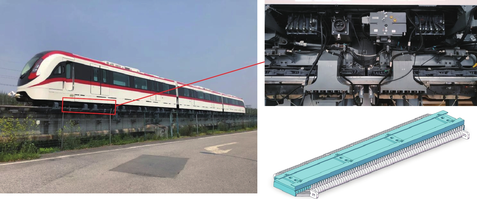
图 1 中低速磁浮列车与直线电机
Figure 1. Medium and low speed maglev trainas well as its linear motor

图 5 不同滑差频率下电机牵引力-间距曲线
Figure 5. Traction force–spacing curves under different slip frequencies
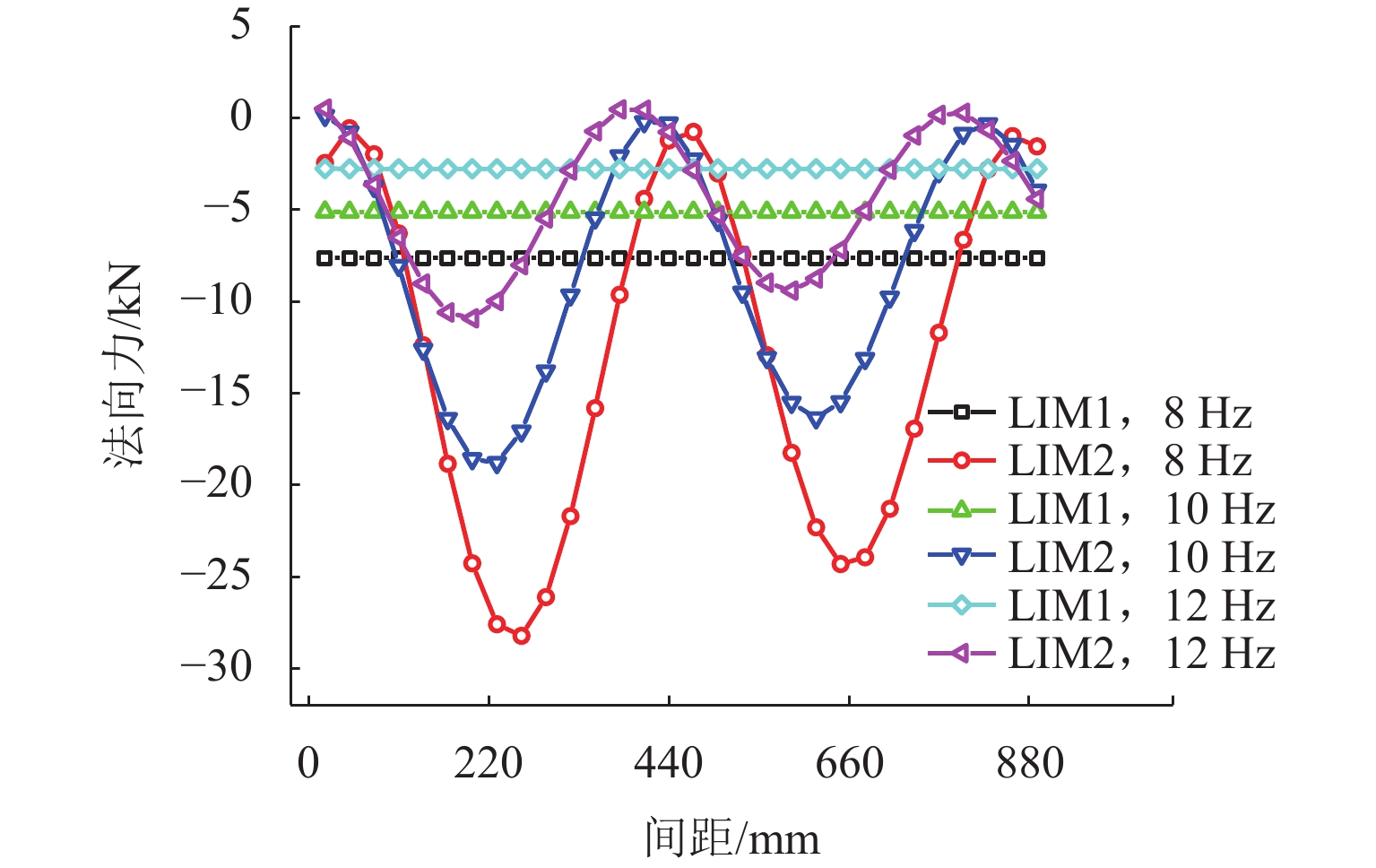
图 6 不同滑差频率下电机法向力-间距曲线
Figure 6. Normal force–spacing curves under different slip frequencies

图 7 不同间距条件下的电机纵向气隙磁密
Figure 7. Magnetic flux density of longitudinal air gap under different spacings
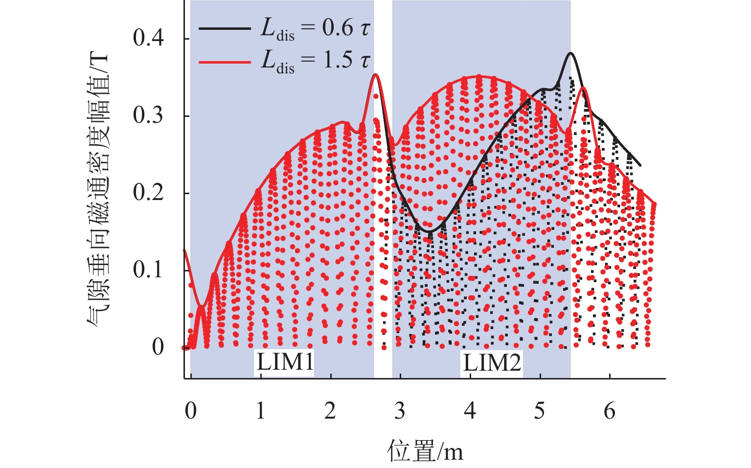
图 8 间距为0.6和1.5倍极距时电机的垂向气隙磁场
Figure 8. Vertical air gap magnetic field at the spacing of 0.6 and 1.5 times pole pitch

图 9 间距为1.2和2.1倍极距时电机的垂向气隙磁场
Figure 9. Vertical air gap magnetic field at the spacing of 1.2 and 2.1 times pole pitch
表 1 电机参数
Table 1. Motor parameters
名称 数值 名称 数值 电机长度/mm 2850 电机容量/(kV•A) 250 电机宽度/mm 220 额定相电压/V 212 极数/极 12 额定相电流/A 400 极距/mm 220 气隙/mm 10 相数 3 滑差频率/Hz 12 每极每相槽数/个 3 单相有效串联匝数/匝 72 次级板电阻率/
(Ω•m)2.83×10⁻⁸ 次级板厚/mm 4  下载: 导出CSV
-
[1] 邓自刚,刘宗鑫,李海涛,等. 磁悬浮列车发展现状与展望[J]. 西南交通大学学报,2022,57(3): 455-474,530. doi: 10.3969/j.issn.0258-2724.20220001DENG Zigang, LIU Zongxin, LI Haitao, et al. Development status and prospect of maglev train[J]. Journal of Southwest Jiaotong University, 2022, 57(3): 455-474,530. doi: 10.3969/j.issn.0258-2724.20220001 [2] 马卫华,胡俊雄,李铁,等. EMS型中低速磁浮列车悬浮架技术研究综述[J]. 西南交通大学学报,2023,58(4): 720-733. doi: 10.3969/j.issn.0258-2724.20210971MA Weihua, HU Junxiong, LI Tie, et al. Summary of suspension frame technology of EMS medium and low speed maglev train[J]. Journal of Southwest Jiaotong University, 2023, 58(4): 720-733. doi: 10.3969/j.issn.0258-2724.20210971 [3] 吴会超,罗建利,周文,等. 中低速磁浮车岔耦合振动研究[J]. 西南交通大学学报,2022,57(3): 483-489. doi: 10.3969/j.issn.0258-2724.20210829WU Huichao, LUO Jianli, ZHOU Wen, et al. Coupled vibration between low-medium speed maglev vehicle and turnout[J]. Journal of Southwest Jiaotong University, 2022, 57(3): 483-489. doi: 10.3969/j.issn.0258-2724.20210829 [4] FRITZ E, WITT M. Maglev train development-history and today’s marketing chances[J]. Elektrische Bahnen, 2012, 110(3): 102-111. [5] BOLDEA I, TUTELEA L N, XU W, et al. Linear electric machines, drives, and MAGLEVs: an overview[J]. IEEE Transactions on Industrial Electronics, 2018, 65(9): 7504-7515. [6] LV G, ZENG D H, ZHOU T, et al. Investigation of forces and secondary losses in linear induction motor with the solid and laminated back iron secondary for metro[J]. IEEE Transactions on Industrial Electronics, 2017, 64(6): 4382-4390. [7] 徐伟,孙广生. 单边直线感应电机纵向边缘效应的研究[J]. 中国工程科学,2007,9(3): 21-27. doi: 10.3969/j.issn.1009-1742.2007.03.004XU Wei, SUN Guangsheng. Research on the longitudinal end effect of single linear induction motor[J]. Engineering Science, 2007, 9(3): 21-27. doi: 10.3969/j.issn.1009-1742.2007.03.004 [8] MISHIMA T, HIRAOKA M, NOMURA T. A study of the optimum stator winding arrangement of LIM in maglev systems[C]//IEEE International Conference on Electric Machines and Drives. San Antonio: IEEE, 2005: 1238-1242. [9] ZHAN J W, LU Q F. Design optimization and performance investigation of novel linear induction motors with V-shaped ladder-slit secondary[J]. International Journal of Applied Electromagnetics and Mechanics, 2018, 58(2): 157-174. doi: 10.3233/JAE-180036 [10] LV G, ZHOU T, ZENG D H, et al. Design of ladder-slit secondaries and performance improvement of linear induction motors for urban rail transit[J]. IEEE Transactions on Industrial Electronics, 2018, 65(2): 1187-1195. [11] LU Q F, LI L X, ZHAN J W, et al. Design optimization and performance investigation of novel linear induction motors with two kinds of secondaries[J]. IEEE Transactions on Industry Applications, 2019, 55(6): 5830-5842. [12] 邓江明,陈特放,唐建湘,等. 单边直线感应电机动态最大推力输出的滑差频率优化控制[J]. 中国电机工程学报,2013,33(12): 123-130,194.DENG Jiangming,CHEN Tefang,TANG Jianxiang,et al. Optimum slip frequency control of maglev single-sided linear induction motors to maximum dynamic thrust[J]. Proceedings of the CSEE,2013,33(12): 123-130,194. [13] 张敏,范屹立,马卫华,等. 滑差频率对磁浮车辆运行性能的影响[J]. 交通运输工程学报,2019,19(5): 64-73. doi: 10.3969/j.issn.1671-1637.2019.05.008ZHANG Min, FAN Yili, MA Weihua, et al. Influence of slip frequency on running performance of maglev vehicle[J]. Journal of Traffic and Transportation Engineering, 2019, 19(5): 64-73. doi: 10.3969/j.issn.1671-1637.2019.05.008 [14] SEO H, LIM J, CHOE G H, et al. Algorithm of linear induction motor control for low normal force of magnetic levitation train propulsion system[J]. IEEE Transactions on Magnetics, 2003, 54(11): 1-4. [15] WANG K, LI Y H, GE Q X, et al. An improved indirect field-oriented control scheme for linear induction motor traction drives[J]. IEEE Transactions on Industrial Electronics, 2018, 65(12): 9928-9937. [16] HAN Y, NIE Z L, XU J, et al. Control strategy for optimising the thrust of a high-speed six-phase linear induction motor[J]. IET Power Electronics, 2020, 13(11): 2260-2268. doi: 10.1049/iet-pel.2019.1334 [17] XIAO X Y, XU W, TANG Y R, et al. Improved loss minimization control based on time-harmonic equivalent circuit for linear induction motors adopted to linear metro[J]. IEEE Transactions on Vehicular Technology, 2023, 72(7): 8601-8612. [18] HU D, XU W, DIAN R J, et al. Loss minimization control of linear induction motor drive for linear metros[J]. IEEE Transactions on Industrial Electronics, 2018, 65(9): 6870-6880. [19] ELMORSHEDY M F, XU W, ALLAM S M, et al. MTPA-based finite-set model predictive control without weighting factors for linear induction machine[J]. IEEE Transactions on Industrial Electronics, 2021, 68(3): 2034-2047. [20] SUN X F, XU J, ZHU J J, et al. Thrust ripple suppression based on negative current control for short-primary low-speed large LIM under transient operation[J]. IEEE Transactions on Energy Conversion, 2023, 38(3): 1566-1575. [21] ZhANG M, LUO S H, GAO C, et al. Research on the mechanism of a newly developed levitation frame with mid-set air spring[J]. Vehicle System Dynamics, 2018, 56(12): 1797-1816. doi: 10.1080/00423114.2018.1435892 [22] ZHANG M, HAN Y P, MA W H, et al. Optimal selection of the linear induction motor spacing for the medium-low speed maglev vehicle[J]. International Journal of Rail Transportation, 2021, 9(2): 157-185. doi: 10.1080/23248378.2020.1742209 [23] 张敏,罗世辉,马卫华. 接线相位差对直线电机牵引性能的影响[J]. 中国科学(技术科学),2019,49(8): 971-980. doi: 10.1360/N092018-00443ZHANG Min, LUO Shihui, MA Weihua. Influence of connection phase difference on the traction performance of linear induction motor[J]. Scientia Sinica (Technologica), 2019, 49(8): 971-980. doi: 10.1360/N092018-00443 [24] 龙遐令. 直线感应电动机的理论和电磁设计方法[M]. 北京:科学出版社, 2006. -

 下载:
下载:


 点击查看大图
计量
- 文章访问数: 396
- HTML全文浏览量: 185
- PDF下载量: 14
- 被引次数: 0