Inversion Method of Vortex-Induced Vibration Amplitude for Long-Span Bridges with Partially Installed Noise Barrier

LI Yongle; PAN Junzhi; TI Zilong; RAO Gang

doi:10.3969/j.issn.0258-2724.20210172

Volume 58 Issue 1

Jan. 2023

Turn off MathJax

Article Contents

Abstract

References

Journal of Southwest Jiaotong University > 2023 > 58(1): 183-190.

LIN Shan, CHEN Jigang, BU Lifeng, ZHANG Wei, CHENG Hongbo. Construction and Application of Intelligent Programming Model for Catenary Maintenance Plan[J]. Journal of Southwest Jiaotong University, 2022, 57(5): 960-966. doi: 10.3969/j.issn.0258-2724.20210034

Citation:

LI Yongle, PAN Junzhi, TI Zilong, RAO Gang. Inversion Method of Vortex-Induced Vibration Amplitude for Long-Span Bridges with Partially Installed Noise Barrier[J]. Journal of Southwest Jiaotong University, 2023, 58(1): 183-190. doi: 10.3969/j.issn.0258-2724.20210172

Citation:

PDF( 3833 KB)

Inversion Method of Vortex-Induced Vibration Amplitude for Long-Span Bridges with Partially Installed Noise Barrier

doi: 10.3969/j.issn.0258-2724.20210172

LI Yongle^1
,,
PAN Junzhi¹,
TI Zilong^{1
,
,},
RAO Gang²

1.
School of Civil Engineering, Southwest Jiaotong University, Chengdu 610031, China
2.
Traffic Construction Engineering Management Center, Luzhou 646000, China

Received Date: 16 Mar 2021
Rev Recd Date: 16 Nov 2021

Available Online: 02 Sep 2022

Publish Date: 18 Nov 2021

Abstract

Abstract

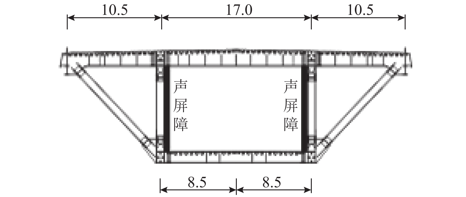
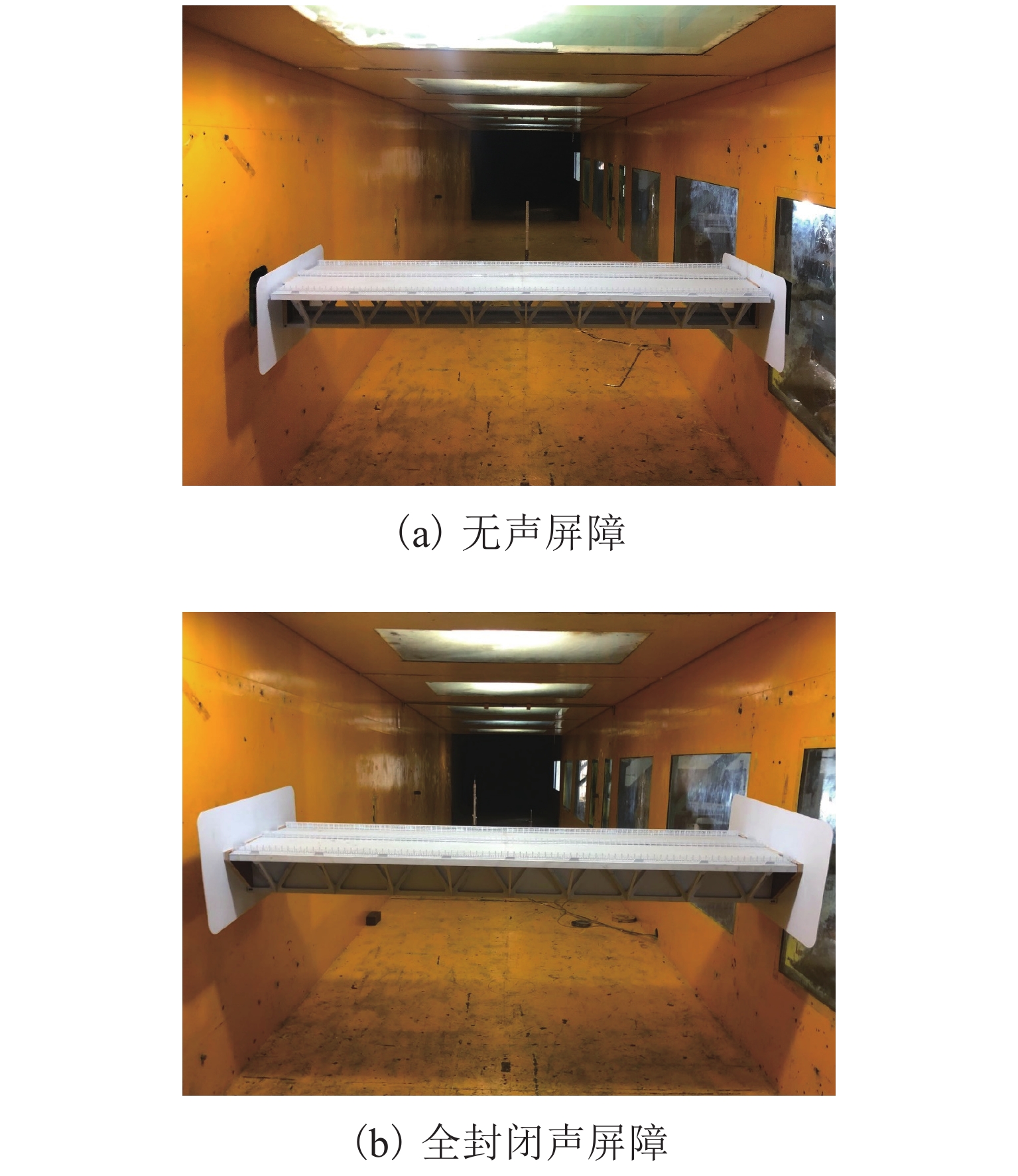
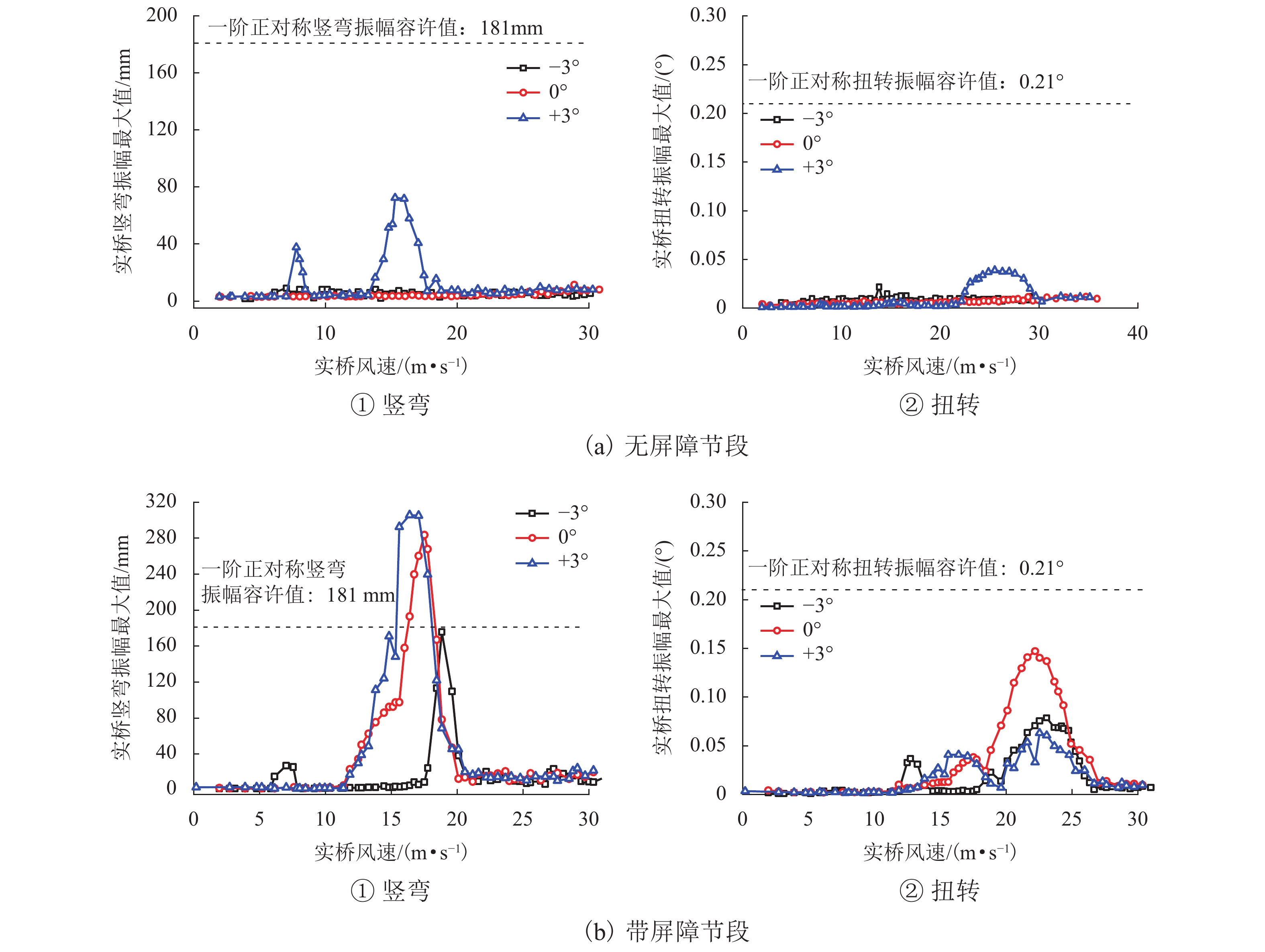
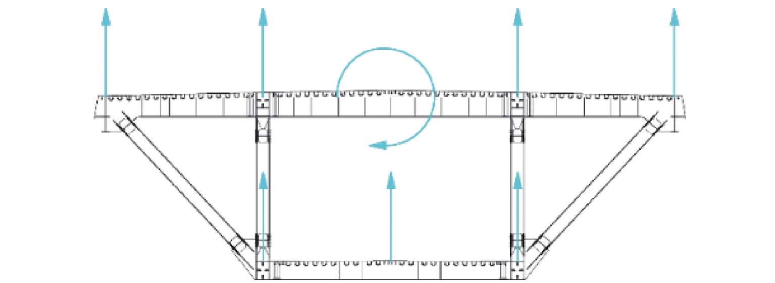
The sectional model test in wind tunnels is often used to measure the vortex-induced vibration (VIV) of long-span bridges. Since the sectional model test is based on two-dimensional theory, when the bridge has different aerodynamic configurations along the span due to the partial installation of noise barriers, it is difficult to measure the VIV response directly through the sectional model test. Based on the empirical linear VIV model, an assessment method of VIV between the sectional model and prototype bridge that considers the effects of multiple aerodynamic configurations is proposed. Firstly, the sectional model test is performed on the models with and without barriers respectively. Then, the prototype response of the noise barriers installed and not installed along the span is investigated by ANSYS harmonic analysis, and the corresponding amplitude of the vortex-induced force is obtained. Finally, according to the actual installation position of the noise barrier along the span, the vortex-induced force is imposed on the bridge and the prototype response with the partially installed noise barrier is obtained. In addition, based on the method in this paper, various noise barrier installation schemes are numerically simulated. The results indicate that fully enclosed noise barrier will significantly reduce the aerodynamic performance of the main girder and the overall VIV will be affected by partial installation of barrier to a large degree. The method in this paper can estimate the prototype response of multi-aerodynamic configurations bridges through the results of sectional model tests. The installation of the noise barrier should be arranged on the side span as far as possible under the conditions of noise reduction. If the arrangement length exceeds the position of the bridge tower, it should be shortened as much as possible to reduce the vortex-induced response.
- long-span bridge,
- vortex-induced vibration (VIV),
- noise barrier,
- sectional model,
- amplitude conversion

FullText(HTML)

随着我国轨道交通的快速发展，轨道交通接触网的规模不断扩大，对接触网运行安全性的要求不断提高，接触网检修作业的任务日渐加重. 科学合理地安排接触网的检修计划，可以有效利用现有检修资源、提高检修作业的效率、节省检修费用，有效保障接触网系统的安全可靠.

现阶段接触网检修计划基本依靠人工编制，由于接触网设备类型多、数量大，设备间关联关系复杂，人工编制检修计划不仅效率低下，而且较难对检修任务做全面考虑，编制的检修计划经济性与可行性较差，容易出现漏修、过修与失修等问题，严重影响了接触网的安全运行. 近年随着信息技术的发展，自动编制技术在铁路行业各领域得到广泛研究与应用，如列车运行图计划编制、线路维修计划编制、编组站计划编制、列车解体计划编制、乘务计划编制、调车作业计划编制等^[1-6]，极大提高了作业任务的合理性与经济性，也为接触网检修任务的自动编制提供了有益的参考.

目前，接触网检修理念研究主要有两类，一是以状态为中心，以设备监测数据为基础，建立劣化模型预测设备状态变化，并据此安排检修任务，文献[7-8]提出将故障预测与健康管理（prognostics health management, PHM）以及主动维护应用于高速铁路牵引供电系统中，实现策略的决策与优化，可根据设备状态按需检修，有效解决了过修或者欠修的不足. 但依据该理念编制检修计划需要大量状态检测与监测数据，同时需要较强的数据实时分析与处理能力，较难直接应用到实际中. 二是以可靠性为中心，通过建立设备寿命分布模型，以此为基础优化检修计划编制，如文献[9-10]针对现有的接触网预防性维修模式，推导了系统可靠性与维修费用的数学关系；文献[11]运用ID3 （iterative dichotmizer 3）决策树算法构建出接触网维修决策树模型，通过决策树发掘影响接触网主要设备异常或故障的主要因素，从而获得相对科学合理的检修方案；文献[12]开发了接触网设备管理子系统以及检修沙盘模型、手持终端子系统，实现了图表可视化、生产作战指挥图和报表定制等功能，但该系统的检修计划依赖人工编制；文献[13-14]获得了各设备的最优维修间隔，并以设备类别为最小单位编制检修计划，但编制结果没考虑接触网设备的位置分布，无法在实际中得到应用.

本文在满足检修作业特性的基础上，针对接触网设备沿线分布、点状与条状设备并存等特性，考虑检修作业的连续性，利用整数规划方法，提出基于弹性周期区间的接触网检修计划自动编制模型，设计相应的启发式求解算法，通过实际算例验证模型和算法的有效性，为铁路接触网检修计划的自动编制提供一种有效方法.

1. 模型构建

1.1 模型相关定义与假设

定义1　接触网检修涉及的所有设备集合称为检修任务集，根据设备在接触网中的位置可划分为线条状全面检修类子集合与点状单项设备类子集合.

定义2　检修任务指接触网设备周期性人工检修，对于设备发生故障或病害后所采取的事后修理（又称为纠错性维修）不属于本文定义的检修任务.

定义3　接触网检修工作量以设备检修次数定义，不考虑不同设备检修时间的差异性问题.

模型假设如下：

1）区域路网中接触网检修设备已确定，模型只需考虑如何安排任务使目标费用最小.

2）所有检修任务集合中的元素在计划时间范围内按照检修周期执行.

3）运营过程中的纠错性维修，不影响计划中检修任务的安排.

1.2 模型框架构建

目前的计划检修体制要求设备到期必修，一般不允许超周期运行. 这样特定的检修方式极大限制了各设备检修过程中实现时空配合的可能性，考虑设备本身具有一定的过载能力，提出一种弹性周期区间的方法，如图1所示.

图 1 弹性周期区间关系示意

Figure 1. Schematic of elastic period interval

下载: 全尺寸图片幻灯片

图1中：T为《普速铁路接触网运行维修规则》^[15]规定的标准检修周期； ${T_{\rm{D}}}$ 为允许过修的编制时间下限； ${T_{\rm{U}}}$ 为允许迟修的编制时间上限. 弹性周期在确保设备可靠性满足要求的情况下，允许一定的过修率和迟检率，从而将设备的检修周期由一个固定的时刻拓展至一个区间，增加了不同设备在时间和空间上配合的可能性. 从而使设备检修计划更加灵活，编制结果更加优化.

接触网检修计划的编制是在给定的任务检修时间内，将需要进行检修的设备进行排列组合，确保检修任务顺利开展，主要目的是通过数学方法解决预防性检修计划编制问题. 检修计划可分解为年度、月度、天窗日计划等，其本质差异仅在于考虑的编制时间段不同，其中年度检修计划是分解编制的基础.

以接触网年度检修计划自动编制为例，模型输入包括设备所处的位置、检修周期等基本信息，模型约束主要包括设备检修优先级约束、线条状设备检修连续性约束等. 基于弹性周期区间的接触网年度检修计划自动编制模型（automatically compilingmodel for overhaul plan of catenary based on elastic period interval，ACM-OPC-EPI）框架如图2所示.

图 2 模型整体框架

Figure 2. Model framework

下载: 全尺寸图片幻灯片

1.3 接触网检修计划优化模型

接触网检修计划编制的目的是在满足设备运行可靠性约束的基础上，希望以最小的检修成本，按要求完成所有接触网设备的检修作业任务.

1） ACM-OPC-EPI目标函数

设备超周期惩罚费用目标F₁和额外检修路径代价目标F₂如式（1）和式（2）所示.

${\rm{min}}\;{F_1} = \sum\limits_{l \in {L_{\rm{C}}}} {\sum\limits_{e \in {D_{\rm{C}}^{(l)}}} {\sum\limits_{t \in {T_{\rm{S}}}} {P_{\rm F}^{(el)}X_t^{(el)}} } },$

(1)

${\rm{min}}\; {F_2} = \sum\limits_{l \in {L_{\rm{C}}}} {\sum\limits_{e \in {D_{\rm{C}}^{(l)}}} {\sum\limits_{t \in {T_{\rm{S}}}} {P^{(el)}_{{\rm{C}}_t}}{X_t^{(el)}} } } ,$

(2)

式中：L_C为工区股道集合，； ${D_{\rm{C}}^{(l)}}$ 为股道l计划内需要安排的设备集合；T_S为计划编制时间区段元素集合， ${T}_{{\rm{S}}}=\left\{1,2,\cdots ,T_{\rm {max}}\right\}$ ，其中， $T_{\rm {max}}$ 为最大编制时间区段数，年度计划中T_max = 12； ${P_{\rm{F}}^{(el)}}$ 为股道l设备e计划内检修超周期惩罚费用； ${P_{{\rm{C}}_t}^{(el)}}$ 为编制时间区段t内股道l设备e因任务分散导致的一次出行额外检修路径代价，即：编制时间区段内单项设备与计划内区域连续性设备的最小杆号差，以此量化单项设备与连续设备的距离； $X_t^{(el)}$ 为作业任务0-1决策变量集，

${X}_{t}^{(el)}=\left\{\begin{array}{ll}\text{1},& 股道\;l\;设备\; e \;被安排在第\; t\;个时间\\& 编制区段,\\ \text{0},& 股道 \;l \;设备\; e \;未被安排在第\; t \;个时\\& 间编制区段.\end{array} \right.$

上述目标中，式（1）表示设备检修间隔偏离标准检修周期最小，以保证标准周期内检修率最大化. 当设备修安排未超周期时，将 $P_{\rm F}^{(el)}$ 置0处理；当设备检修安排超周期时，惩罚费用如下式所示：

${P}_{{\rm{F}}}^{(el)}=\left\{ \begin{array}{l}0, \;\;\;\; {D}_{{\rm{L}}}{E}_{{\rm{C}}}^{(el)}\leqslant {t}^{(el)}-{t}_{{\rm{p}}}^{(el)} < {E}_{{\rm{C}}}^{(el)},\\ \dfrac{{t}^{(el)}-{t}_{{\rm{p}}}^{(el)}-{E}_{{\rm{C}}}^{(el)}}{{E}_{{\rm{C}}}^{(el)}}, \;\;\;\; {E}_{{\rm{C}}}^{(el)}\leqslant {t}^{(el)}-{t}_{{\rm{p}}}^{(el)} < {U}_{\rm L}{E}_{{\rm{C}}}^{(el)},\end{array}\right.$

式中： ${t^{(el)}}$ 为股道l设备e在本次检修时间范围的自身周期内设备编制执行的时间点； ${t_{\rm{p}}^{(el)}}$ 为股道l设备e在上一计划编制时间范围内最后一次检修执行时间点以及本次编制时间范围内上一设备编制周期的检修执行时间点； ${E_{\rm{C}}^{(el)}}$ 为股道l设备e检修标准周期； ${U_{ \rm{L}}}$ 为弹性编制周期上限因子； ${D_{\rm{L}}}$ 为弹性编制周期下限因子.

式（2）描述了各时间编制区段检修任务编制的集中性.

2） ACM-OPC-EPI约束条件

设备弹性周期编制区间约束如式（3）所示.

$\sum\limits_{{t^{(el)}} = {{t^{(el)} _{\rm{p}}}+ {D_{\rm{L}}}{E^{(el)}_{\rm{C}}} }}^{ {{t_{\rm{p}}^{(el)} }+ {U_{\rm{L}}}{E_{\rm{C}}^{(el)}} }} {X_t^{(el)} = 1},$

(3)

式中： ${t \in {T_{\rm{S}}}}； e \in {D_{\rm{C}}^{(l)} }$ ； ${U_{\rm{L}}}{E^{(el)}_{\rm{C}}}$ 对应图1中的编制时间上限T_U； ${D_{\rm{L}}}{E_{\rm{C}}^{(el)} }$ 对应图1中的编制时间下限T_D.

检修工作量约束如式（4）和式（5）所示.

$\sum\limits_{l \in {L_{\rm{C}}}} {\sum\limits_{e \in {D_{\rm{C}}^{(l)}}} {\sum\limits_{t \in {T_{\rm{S}}}} {X_t^{(el)}} } } \leqslant 1.{\text{05}}{N_{{t}}},$

(4)

$\sum\limits_{l \in {L_{\rm{C}}}} {\sum\limits_{e \in {D_{\rm{C}}^{(l)}}} {\sum\limits_{t \in {T_{\rm{S}}}} {X_t^{(el)}} } } \geqslant {\text{0}}{\text{.95}}{N_{{t}}},$

(5)

式中： ${N_t}$ 为第 $t$ 个时间编制区段计划编制工作量，具体描述为各时间编制区段检修能力由于天气、温度，以及客流量（春运、暑运）等外部条件影响，造成在各个时间编制区段具有差异性，通过此约束可确定每个检修区段的检修工作量上下限约束.

设备编制优先级约束如式（6）所示.

$\left\{ {\begin{array}{*{20}{l}} {{F_{\rm{R}}^{(el)}}} > {F_{\rm{R}}^{((e + {\text{1}})l)}},\quad {P_{\rm{F}}^{(el)}}> {P_{\rm{F}}^{((e+1)l)}} , \\ {{F_{\rm{R}}^{(el)} }} < {F_{\rm{R}}^{((e + {\text{1}})l)}},\quad {P_{\rm{F}}^{(el)}}< {P_{\rm{F}}^{((e+1)l)}} , \end{array}} \right.$

(6)

式中： ${\text{ }}l \in {L_{\rm{C}}}；\;e,(e + 1) \in {L_{\rm{D}}^{(l)}}$ ， ${L_{\rm{D}}^{(l)}}$ 为股道l计划内需要安排的线条状全面检修类设备集合； ${F_{\rm{R}}^{(el)}}$ 为股道l设备e检修首次周期内编制优先级标号，依据接触网检修规程，漏修失修设备大于正常设备、单项设备优先级大于线索类设备，如下式所示.

${F_R^{(el)}} = \left\{ {\begin{array}{*{20}{l}} {2,\;\;\;\;{t_{{\rm{Ls}}}} - {t_{\rm{p}}^{(el)}} > {U_{\rm{L}}}{E_{\rm{C}}^{(el)}},{\text{ }}e \in {P_{\rm{D}}^{(l)}}} ,\\ {1,\;\;\;\;{t_{\rm{L}}}_{\rm{s}} - {t_{\rm{p}}^{(el)}} > {U_{\rm{L}}}{E_{\rm{C}}^{(el)}},{\text{ }}e \in {L_{\rm{D}}^{(l)}}}, \\ {0,\;\;\;\;{t_{\rm{L}}}_{\rm{s}} - {t_{\rm{p}}^{(el)}} \leqslant {U_{\rm{L}}}{E_{\rm{C}}^{(el)}},{\text{ }}e \in {D_{\rm{C}}^{(l)}}} , \end{array}} \right.$

式中： ${t_{\rm{L}}}_{\rm{s}}$ 为计划编制起始时间点； ${P_{\rm{D}}^{(l)}}$ 为股道l计划内需要安排的点状单项设备类设备集合.

线条状设备杆号区域连续性约束和连续区间设备数量的最小值约束分别如式（7）和式（8）所示.

$P_t^{((e + {\text{1}})l)}X_t^{((e + {\text{1}})l)} - P_t^{(el)}X_t^{(el)} \leqslant {\text{2}},$

(7)

${\text{max }}\{P_t^{(el)}{\text{}}X_t^{(el)}{\text{}}\} - {\text{min }}\{P_t^{(el)}{\text{}}X_t^{(el)}{\text{}}\} > {R_{\rm{C}}} ,$

(8)

式中： $l \in {L_{\rm{C}}}；\,e,(e + 1) \in {L^{(el)}_{{\rm X}t}}$ ， ${L^{(el)}_{{\rm{X}}t}}$ 为编制时间区段t内设备集合股道l中线条状设备子集； $P_t^{(el)}$ 为编制时间区段t内股道l设备e杆号标识； ${R_{\rm{C}}}$ 为区域最小连续杆号检修工作量.

计划编制时间范围内设备是按频次的周期检修如式（9）所示.

$X_t^{(el)} = X_{t + z{E_{\rm{C}}^{(el)}}}^{(el)},$

(9)

式中： $l \in {L_{\rm{C}}}； e \in {D_{\rm{C}}^{(l)}} ；{\text{1}} \leqslant t{\text{ < }}{T_{\rm{max}}}；{\textit{z}} \in \{{{\text{0,1,}} \cdots, } {F^{(el)}}-1\}$ ， ${F^{(el)}}$ 为股道l设备e计划内检修的执行频次，

$\begin{gathered} {F^{(el)}} = \left\{ {\begin{array}{*{20}{l}} {\left\lceil {\dfrac{{{T_{\rm L}}}}{{{E_{\rm{C}}^{(el)}}}}} \right\rceil , \;\;\;\; {D_{\rm{L}}}{E_{\rm{C}}^{(el)}} \leqslant {t^{(el)}} - {t_{\rm{p}}^{(el)}} < {E_{\rm{C}}^{(el)}}}, \\ {0, \;\;\;\; {E_{\rm{C}}^{(el)}} \leqslant {t^{(el)}} - {t_{\rm{p}}^{(el)}} < {U_{\rm{L}}}{E_{\rm{C}}^{(el)}} , } \end{array}} \right. \end{gathered}$

式中： ${\text{ }}l \in {T_{\rm{C}}}； e \in {D_{\rm{C}}^{(l)}}$ ； ${T_{\rm{L}}}$ 为计划编制时间范围， ${T_{\rm{L}}} = {t_{\rm{L}}}_{\rm{e}} - {t_{\rm{L}}}_{\rm{s}}$ ， ${t_{\rm{L}}}_{\text{e}}$ 为计划编制结束时间点.

2. 启发式求解算法

接触网检修计划需同时满足超周期惩罚费用最小与检修路径代价最小两个目标，结合多目标规划中的分层序列法思想，提出了求解ACM-OPC-EPI模型的启发式算法，算法流程如图3所示.

图 3 ACM-OPC-EPI启发式算法流程

Figure 3. Flow chart of ACM-OPC-EPI heuristic algorithm

下载: 全尺寸图片幻灯片

求解ACM-OPC-EPI模型的启发式算法原则如下：

1）接触网检修计划的编制应优先考虑检修周期问题，设备检修必须处于弹性检修周期之内，以确保接触网运行的安全性.

2）其次考虑接触网线条状设备与点状设备并存的情况，在编制过程中考虑点状设备与线条状设备之间的空间距离问题，使计划编制结果在空间上尽量集中，以节省检修时间与出行费用，确保检修计划编制的经济性.

3. 算例验证分析

3.1 算例描述

某供电工区所辖设备情况如表1所示，其中线条状连续设备包括接触悬挂、附加悬挂、所亭供电线，点状单项设备包括分段绝缘器、关节式分相/分相绝缘器、远动隔离开关及操作机构、避雷器及接地装置，合计作业任务检修6333台次. 各设备标准检修周期参考《普速铁路接触网运行维修规则》^[15].

表 1 检修设备细目表

Table 1. Detailed maintenance equipment information

设备类型	设备名称		标号	单位	周期
线条状设备全面检修	接触悬挂		A	条•km	36 月
	附加悬挂	回流线		条•km	36 月
		架空地线		条•km	36 月
		加强线		条•km	36 月
	所亭供电线	供电线		条•km	36 月
	所亭供电线	架空地线		条•km	36 月
点状单项设备检修	分段绝缘器		B1	组	6 月
	关节式分相、分相绝缘器		B2	组	6 月
	远动隔离开关及操作机构		B3	台	6 月
	避雷器及接地装置		B4	台	12 月

下载: 导出CSV

| 显示表格

设置区域最小连续杆号检修工作量 ${R_{\rm{C}}}$ 为80，弹性编制周期上、下限因子分别取1.2与0.8，考虑不同月份环境的影响，各月可完成的工作量不同，各月可完成的检修工作量比率设置如表2所示. 可从设备检修管理信息系统数据库查询得到设备历史检修信息.

表 2 月检修工作量编制比率

Table 2. Monthly maintenance workload ratio

T_S	1 月	2 月	3 月	4 月	5 月	6 月	7 月	8 月	9 月	10 月	11 月	12 月
比率/%	5	5	15	8	8	15	6	6	10	10	6	6

下载: 导出CSV

| 显示表格

3.2 模型求解结果

求解结果以平铺计划表形式展示如表3，表中垂直方向表示编制区间的计划时段（1月—12月），水平方向上分为线条状设备以及单项设备（其中，A、B1 ~ B4表示设备编号），线条状以连续杆号区间形式进行平铺展示（例：892 ~ 946），单项设备以设备类别进行杆号单独显示（例：266，268，…），其中线条状设备的检修台次以设备履历表中杆号区间包含的设备进行统计（即“/”后的数字，例：/91）. 由结果可以看出：各编制区间检修工作计划符合各约束条件，线条状设备与单项设备在空间位置上普遍集中，符合实际需求.

表 3 编制结果平铺计划

Table 3. Schedule generated with compilation results

编制时间段	股道 L1					股道 L2					月检/ 台次
编制时间段	A	B1	B2	B3	B4	A	B1	B2	B3	B4	月检/ 台次
1 月	892 ~ 946 /91 1052 ~ 1082 /96				898，1004	553 ~ 635 /134				561	324
2 月	260 ~ 360 /165		266，268， 270，272， 274，276， 278，280	264，268， 278，284	262，284， 350	259 ~ 353 /150		265，267， 269，271， 273，275， 277，279	263，267，277，281， 285	261，283， 349	346
3 月	362 ~ 474 /285 520 ~ 672 /273				562	355 ~ 457 /260 877 ~ 945 /126				897	946
4 月	674 ~ 816 /262				770	459 ~ 501 /86 771 ~ 829 /150				487，769	501
5 月	948 ~ 982 /82 818 ~ 890 /185					947 ~ 1001 /122 831 ~ 875 /115	1305				505
6 月	984 ~ 1050 /184 1084 ~ 1178 /288	1494		1590		637 ~ 769 /201 1003 ~ 1089 /264			1487	1003	941
7 月	1180 ~ 1212 /102					503 ~ 551 /125 1155 ~ 1203 /150		265，267， 269，271， 273，275， 277，279	263，267，267，281， 285		390
8 月	1214 ~ 1258 /138					1205 ~ 1283 /240					378
9 月	476 ~ 518 /86 1260 ~ 1320 /186		266，268， 270，272， 274，276， 278，280	264，268， 278，284	488	1091 ~ 1153 /192 1285 ~ 1333 /150					627
10 月	1372 ~ 1496 /378					1335 ~ 1415 /246	1305				625
11 月	1322 ~ 1370 /150					1417 ~ 1491 /222			1487		373
12 月	1498 ~ 1590 /178	1494		1590	1488	1493 ~ 1589 /196					377
年检/ 台次	3129	2	16	10	9	3129	2	16	12	8	6333

下载: 导出CSV

| 显示表格

该部分计划采用人工编制时需要7 d左右，而采用本文方法后求解时间仅135 s，比原来方法节省99.98%，速度远高于人工编制；原来人工编制的检修计划检修路径总里程为858.0 km, 本文方法生成的检修计划检修路径总里程为573.5 km，检修路径比原来减少33.16%，在同样完成设备检修任务的情况下，降低了检修成本.

4. 结　论

1）针对接触网检修作业设备多、地理位置分散、单项的点状设备与线索的条状设备并存的特点，提出一种接触网检修计划智能编制方法，可在给定接触网检修范围的基础上，实现接触网检修计划的自动编制，与现行的人工编制方法相比，速度快、效率高.

2）接触网检修计划的智能编制方法，以弹性检修周期区间为基础，以检修作业出行路径和超周期检修时间总数最小为目标，可实现所辖接触网设备检修计划的自动编制，避免超修和漏修的情况.

3）以某供电分区接触网设备检修计划为例，实现了该工区接触网设备检修计划的自动编制，得到了该工区接触网年度检修的平铺计划表. 计划编制用时短、覆盖设备全面，编制结果满足现场实际检修作业的需要.

致谢：广东省城市轨道交通工程建造新技术企业重点实验室资助（2017B030302009）.

References(16)

References

[1]	苏洋. 公铁两用双层桥梁风屏障气动机理及优化研究[D]. 成都: 西南交通大学, 2017.
[2]	韩旭,彭栋,向活跃,等. 横风作用下高速铁路桥梁全封闭声屏障气动特性的风洞试验研究[J]. 铁道建筑,2019,59(7): 151-155. doi: 10.3969/j.issn.1003-1995.2019.07.35 HAN Xu, PENG Dong, XIANG Huoyue, et al. Research on wind tunnel tests for aerodynamic characteristics of closed noise barriers on high speed railway bridges under crosswinds[J]. Railway Engineering, 2019, 59(7): 151-155. doi: 10.3969/j.issn.1003-1995.2019.07.35
[3]	孙延国,廖海黎,李明水. 基于节段模型试验的悬索桥涡振抑振措施[J]. 西南交通大学学报,2012,47(2): 218-223,264. doi: 10.3969/j.issn.0258-2724.2012.02.008 SUN Yanguo, LIAO Haili, LI Mingshui. Mitigation measures of vortex-induced vibration of suspension bridge based on section model test[J]. Journal of Southwest Jiaotong University, 2012, 47(2): 218-223,264. doi: 10.3969/j.issn.0258-2724.2012.02.008
[4]	SIMIU E S R H. Wind effects on structures[M]. New York: Wiley, 1986.
[5]	EHSAN F, SCANLAN R H. Vortex-induced vibrations of flexible bridges[J]. Journal of Engineering Mechanics, 1990, 116(6): 1392-411. doi: 10.1061/(ASCE)0733-9399(1990)116:6(1392)
[6]	HARTLEN R T, CURRIE IAIN G. Lift-oscillator model of vortex-induced vibration[J]. Journal of the Engineering Mechanics Division, 1970, 96(5): 577-91. doi: 10.1061/JMCEA3.0001276
[7]	周帅,陈克坚,陈政清,等. 大跨桥梁涡激共振幅值估算方法的理论基础与应用[J]. 高速铁路技术,2019,10(5): 25-31. doi: 10.12098/j.issn.1674-8247.2019.05.006 ZHOU Shuai, CHEN Kejian, CHEN Zhengqing, et al. Theoretical basis and practical applications of various vortex-induced vibration amplitudes estimation methods for large-span bridges[J]. High Speed Railway Technology, 2019, 10(5): 25-31. doi: 10.12098/j.issn.1674-8247.2019.05.006
[8]	张志田,陈政清. 桥梁节段与实桥涡激共振幅值的换算关系[J]. 土木工程学报,2011,44(7): 77-82. doi: 10.15951/j.tmgcxb.2011.07.009 ZHANG Zhitian, CHEN Zhengqing. Similarity of amplitude of sectional model to that of full bridge in the case of vortex-induced resonance[J]. China Civil Engineering Journal, 2011, 44(7): 77-82. doi: 10.15951/j.tmgcxb.2011.07.009
[9]	周奇,孟晓亮,朱乐东. 基于非线性涡激力广义模型的涡振幅值换算[J]. 土木工程学报,2020,53(10): 82-88. doi: 10.15951/j.tmgcxb.2020.10.008 ZHOU Qi, MENG Xiaoliang, ZHU Ledong. Amplitude conversion of vortex-induced vibration based on generalized model of nonlinear vortex-induced force[J]. China Civil Engineering Journal, 2020, 53(10): 82-88. doi: 10.15951/j.tmgcxb.2020.10.008
[10]	SUN Y G, LI M S, LIAO H L. Nonlinear approach of vortex-induced vibration for line-like structures[J]. Journal of Wind Engineering and Industrial Aerodynamics, 2014, 124: 1-6. doi: 10.1016/j.jweia.2013.10.011
[11]	IRWIN P. Full aeroelastic model tests[M]. [S.l.]: Routledge, 2017: 125-35.
[12]	HJORTH-HANSEN E. Section model tests[M]. [S.l.]: Routledge, 2017: 95-112.
[13]	秦浩,廖海黎,李明水. 变截面连续钢箱梁桥典型施工阶段涡激振动[J]. 西南交通大学学报,2014,49(5): 760-765,786. doi: 10.3969/j.issn.0258-2724.2014.05.003 QIN Hao, LIAO Haili, LI Mingshui. Vortex-induced vibration of continuous steel box-girder bridge with variable cross-sections at typical erection stages[J]. Journal of Southwest Jiaotong University, 2014, 49(5): 760-765,786. doi: 10.3969/j.issn.0258-2724.2014.05.003
[14]	DUAN J L, HUANG W P. CFD-based numerical analysis of a variable cross-section cylinder[J]. Journal of Ocean University of China, 2014, 13(4): 584-588. doi: 10.1007/s11802-014-2048-0
[15]	陈政清. 工程结构的风致振动、稳定与控制[M]. 北京: 科学出版社, 2013.
[16]	王新敏. ANSYS结构动力分析与应用 [M]. 北京: 人民交通出版社, 2014.

Relative Articles

[1]	YANG Meng, WANG Yunfei, ZHAO Jiabin, ZHOU Jing, WANG Yongjing, LI Yongle. Vortex-Induced Vibration Response of Bridges Considering Both Spanwise Variation of Vibration Amplitude and Correlation of Aerodynamic Forces[J]. Journal of Southwest Jiaotong University, 2025, 60(1): 45-52. doi: 10.3969/j.issn.0258-2724.20220714
[2]	HUANG Lin, DONG Jiahui, LIAO Haili, PU Shiyu, WANG Qi. Vortex-Induced Vibration (VIV) Aerodynamic Measures of Girder with Side Beam Based on Computation Fluid Dynamics (CFD) and Wind Tunnel Test[J]. Journal of Southwest Jiaotong University, 2024, 59(2): 343-352. doi: 10.3969/j.issn.0258-2724.20220208
[3]	WANG Yawei, ZHU Jin, ZHENG Kaifeng, SU Yonghua, GUO Hui, LI Yongle. Coupled Vibration Analysis of Earthquake-Wind-Vehicle-Bridge for Long-Span Bridges Considering Scouring Effect[J]. Journal of Southwest Jiaotong University, 2024, 59(2): 323-331. doi: 10.3969/j.issn.0258-2724.20220091
[4]	WEI Xing, WANG Rongrong, WEN Zongyi, DAI Lijun, HU Zhe. Influence of Bolt Relaxation of High-Speed Railway Sound Barrier on Fatigue Life[J]. Journal of Southwest Jiaotong University, 2023, 58(2): 373-380. doi: 10.3969/j.issn.0258-2724.20210060
[5]	HUANG Lin, DONG Jiahui, WANG Qi, LIAO Haili. Influence of Maintenance Rail Position and Guide Vanes on Vortex-Induced Vibration Performance of Flat Box Girders[J]. Journal of Southwest Jiaotong University, 2023, 58(3): 535-545. doi: 10.3969/j.issn.0258-2724.20210474
[6]	WEI Xing, ZHANG Jing, WEI Huanbo, HU Zhe, WEN Zongyi. Structural Effect on Mechanical Behavior of High-Speed Railway Sound Barriers Based on Vibration Response[J]. Journal of Southwest Jiaotong University, 2022, 57(2): 353-359, 409. doi: 10.3969/j.issn.0258-2724.20200243
[7]	LI Ming, SUN Yanguo, LI Mingshui, WU Bo. Vortex-Induced Vibration Performance of Wide Streamlined Box Girder and Aerodynamic Countermeasure Research[J]. Journal of Southwest Jiaotong University, 2018, 53(4): 712-719. doi: 10.3969/j.issn.0258-2724.2018.04.007
[8]	ZHENG Shixiong, GUO Junfeng, ZHU Jinbo, TANG Yu. Characteristics and Suppression Neasures for Soft Flutter of Main Girder with П-Shaped Cross Section[J]. Journal of Southwest Jiaotong University, 2017, 30(3): 458-465. doi: 10.3969/j.issn.0258-2724.2017.03.004
[9]	LIU Jun, LIAO Haili, WAN Jiawei, MA Cunming. Effect of Guide Vane beside Maintenance Rail on Vortex-Induced Vibration of Streamlined Box Girder[J]. Journal of Southwest Jiaotong University, 2015, 28(5): 789-795. doi: 10.3969/j.issn.0258-2724.2015.05.004
[10]	LUO Gang, ZHOU Xiaojun. Vortex-Induced Fatigue Damage Analysis of Submerged Floating Tunnel Cable[J]. Journal of Southwest Jiaotong University, 2014, 27(4): 642-648. doi: 10.3969/j.issn.0258-2724.2014.04.013
[11]	QIN Hao, LIAO Haili, LI Mingshui. Vortex-Induced Vibration of Continuous Steel Box-Girder Bridge with Variable Cross-Sections at Typical Erection Stages[J]. Journal of Southwest Jiaotong University, 2014, 27(5): 760-765,786. doi: 10.3969/j.issn.0258-2724.2014.05.003
[12]	ZHOU Xin, XIAO Xinbiao, HE Bin, HAN Jiaqi, WEN Zefeng, JIN Xuesong. Influential Factors and Rules for Insertion Loss of High-Speed Railway Noise Barriers[J]. Journal of Southwest Jiaotong University, 2014, 27(6): 1024-1031. doi: 10.3969/j.issn.0258-2724.2014.06.014
[13]	SUN Yanguo, LIAO Haili, LI Mingshui. Mitigation Measures of Vortex-Induced Vibration of Suspension Bridge Based on Section Model Test[J]. Journal of Southwest Jiaotong University, 2012, 25(2): 218-223. doi: 10.3969/j.issn.0258-2724.2012.02.008
[14]	SUO Qifeng, LI Mingshui, HE Xiangdong. Effects of 3D Wind Flow on Drag Coefficients of Stay Cables[J]. Journal of Southwest Jiaotong University, 2010, 23(6): 882-887. doi: 10.3969/j.issn.0258-2724.2010.06.010
[15]	L? Jianpin, ZHANG Jiwen, LIAO Jianzhou, HU Weinan, TU Yongming. Response of Noise Barrier for Existing Railway Bridges under Impulsive Pressure Induced by High-Speed Train[J]. Journal of Southwest Jiaotong University, 2009, 22(4): 547-551.
[16]	XIAN Rong, LIAO Haili, LI Mingshui. Calculation of Spanwise Vortex-Induced Vibration Responses of Long-Span Bridge Girder[J]. Journal of Southwest Jiaotong University, 2008, 21(6): 740-746.
[17]	JIAO Changzhou, GAO Bo, WANG Guangdi. Vibration Analysis of Noise Barrier Structures Subjected to Train-Induced Impulsive Wind Pressure[J]. Journal of Southwest Jiaotong University, 2007, 20(5): 531-536.
[18]	WANG Shao-jia, GAO Shu-ying. Predication of Efficiency of Railway Anti-Noise Barriers with Statistical Energy Analysis Method[J]. Journal of Southwest Jiaotong University, 2001, 14(6): 645-647.
[19]	LIU Shan-hong, HE Guang-han. Test Study on Segmental Model of a PPC Box Girder[J]. Journal of Southwest Jiaotong University, 2001, 14(5): 491-494.
[20]	TANGHuai-ping, WANG Feng-qin. Self-Vibration Characteristic Test of Long-Span Bridges by Means of Environment Random Excitation[J]. Journal of Southwest Jiaotong University, 2000, 13(2): 126-128.

Supplements(0)

Cited By

Cited by

Periodical cited type(4)

1.	孙颢，郭国和，朱青，朱乐东，檀忠旭，权红烈. 黄茅海大桥扭转涡振气动措施展向布局优化. 中国公路学报. 2024(10): 98-106 .
2.	游衡锐，遆子龙，李永乐，杨凌，潘俊志. 大跨协作体系桥梁吊跨比对主梁涡振性能的影响. 哈尔滨工业大学学报. 2024(11): 72-79 .
3.	张明金，颜庭辕，胡博，陈红宇，李永乐. 复杂山区桥址区地形模型的边界过渡段线型. 西南交通大学学报. 2024(06): 1423-1430 . 本站查看
4.	遆子龙，杨凌，李永乐，潘俊志. 全封闭式屏障对大跨双层公铁两用悬索桥抗风性能的影响研究. 铁道技术标准(中英文). 2023(06): 33-41 .

Other cited types(3)

Proportional views

Proportional views

通讯作者: 陈斌, bchen63@163.com

1.
沈阳化工大学材料科学与工程学院沈阳 110142

Figures(8) / Tables(2)

Get Citation

PDF

XML

Article views(451) PDF downloads(28)